UNAGI: custom channel model
Brief overview and sample outputs
UNAGI (naming based on EEL which was original due to Marina Levy) is a re-entrant \(\beta\)-plane channel with temperature as the thermodynamic variable that is largely based on Dave Munday’s MITgcm channel model reported in [MJM15], as an idealised model to the Antarctic Circumpolar Current. The model at present takes in some to-be specified bathymetry, wind stress profile and initial state, which may be customised accordingly within the gen_UNAGI_fields.ipynb, which may be found at the host GitHub repository.
With the choice of SST restoring over the surface layer, to maintain a sensible thermocline the vertical tracer diffusivity is enhanced in a sponge region to the north (see [MJM15]). See e.g. [AMF11] for alternative model formulations. Some model set up choices:
relatively long re-entrant zonal channel, no topography except ridge in the middle of the channel extending up to half the depth of the domain
fixed sinusoidal wind stress with some peak wind stress value \(\tau_0\)
SST restoring (a relatively hard restoring, the
rn_dqdtvalue innamelist_cfghas been amplified by a factor of 2)linearly varying temperature profile at the surface with \(e\)-folding depth of 1000 metres
linear friction
linear EOS with only temperature as the thermodynamic variable
sponge region to the north where vertical diffusivity is amplified by a factor of 250 from the background value of \(10^{-5}\ \mathrm{m}^2\ \mathrm{s}^{-1}\)
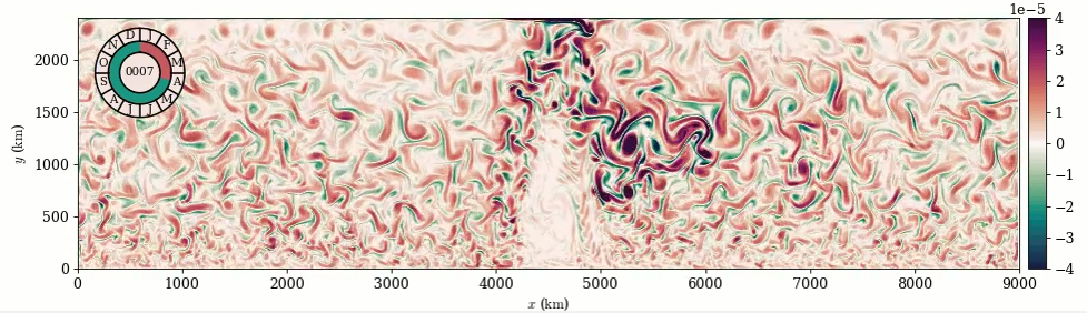
The diagram below shows the surface relative vorticity (in units of \(\mathrm{s}^{-1}\)) from the 10km resolution model with biharmonic tracer diffusion and no eddy parameterisation, associated with a rich eddying field. Click here for an animation.
How to get the model running
If you just want things to work then try the zenodo repository, which has all the NEMO modified sources files and model input files required. Some sample analysis code are given in host GitHub repository.
It is also fairly quick to recreate the forcing files from scratch, and is likely more informative for making your own models. The relevant notebook is gen_UNAGI_fields.ipynb, given also in host GitHub repository. The code can almost be run straight except for one step; see below notes.
Building the custom model
The following approach is strictly for NEMO models beyond v3.6, where one can build a customised model through providing a domcfg.nc, which is the main goal here. The details are given below are what I did for the idealised channel model UNAGI; see here for a step-by-step guide of how I did it.
The biggest obstacle in generating the appropriate domcfg.nc file for me was in transferring the code that modifies the vertical spacing variables e3t/u/v/w to have a partial cell description. I first tried to brute force it by writing from scratch a file that provides all the relevant variables needed in the domcfg.nc; see for example the input required in ORCA2. I gave up after a while and fell back to using the NEMO native [MI96] grid and the TOOLS/DOMAINcfg package, as follows:
in an external folder (e.g.,
~/Python/NEMO/UNAGI), create the bathymetry data through a program of your choice (e.g. Python), and output it as a netCDF file (e.g.bathy_meter.nc)link/copy it as
bathy_meter.nc(the tool requires that specific naming) into theTOOLS/DOMAINcfgthat comes with NEMOmodify the
namelist_cfgfile accordingly for the horizontal and vertical grid spacing parameters (see here for usage and compiling notes), and the one I used for this model is given as an example in that packages pagea
domcfg.ncshould result (if not, seeocean.outputfor messages), copy it back into the working folder in step 1open
domcfg.ncand use those variables to create thestate.ncandforcing.ncfile again in the program of your choice (this is mostly to keep consistency; I did it in Python)copy the
domcfg.nc,state.ncandforcing.nc(I prefixed them with something, e.g.UNAGI_domcfg_R010.nc) and modify thenamelist_cfgaccordingly, e.g.
!-----------------------------------------------------------------------
&namrun        !   parameters of the run
!-----------------------------------------------------------------------
   cn_exp      =      "UNAGI" !  experience name
   nn_it000    =          1   !  first time step
   nn_itend    =       8640   !  last  time step
   nn_date0    =      10101   !
   nn_leapy    =         30   !  Leap year calendar (1) or not (0)
   ln_rstart   = .false.   !  start from rest (F) or from a restart file (T)
      nn_euler    =    1            !  = 0 : start with forward time step if ln_rstart=T
      nn_rstctl   =    0            !  restart control ==> activated only if ln_rstart=T
      !                             !    = 0 nndate0 read in namelist
      !                             !    = 1 nndate0 check consistancy between namelist and restart
      !                             !    = 2 nndate0 check consistancy between namelist and restart
   nn_stock    =       8640   !  frequency of creation of a restart file (modulo referenced to 1)
   nn_write    =       8640   !  frequency of write in the output file   (modulo referenced to nn_it000)
/
!-----------------------------------------------------------------------
&namcfg     !   parameters of the configuration
!-----------------------------------------------------------------------
   ln_read_cfg = .true.    !  (=T) read the domain configuration file
      !                    !  (=F) user defined configuration  ==>>>  see usrdef(_...) modules
      cn_domcfg = "domcfg_UNAGI" ! domain configuration filename
/
...
That is more or less it. Once you can build the domain variables the model will at least run and the rest is more to do with experimental design.
Hacking NEMO to get UNAGI
That two main things that needed hacking into NEMO for UNAGI are the vertical tracer diffusion (in the sponge region to the north) and possible combination with the GEOMETRIC parameterisation, the latter could be found here. For the vertical tracer diffusion given in zdfphy.f90, I hacked an existing variable so that it is dual use to give a specified meridional profile in the vertical diffusivity; search for the variable rn_avt_amp in this file to see how I did it.
An extra hack I did was to shut off a default warning in ldftra.f90 (with modifications to trazdf.f90 for completeness) that biharmonic tracer diffusion cannot be used with when the GM scheme (ldfeiv) is used. Normally if you are using GM you also use isoneutral diffusion rather than biharmonic diffusion, but for my case I do intend on having that specific combination.
- AMF11
R. Abernathey, J. Marshall, and D. Ferreira. The dependence of Southern Ocean meridional overturning on wind stress. J. Phys, Oceanogr., 41:2261–2278, 2011. doi:10.1175/JPO-D-11-023.1.
- MI96
G. Madec and M. Imbard. A global ocean mesh to overcome the North Pole singularity. Clim. Dyn., 12:381–388, 1996. doi:10.1007/BF00211684.
- MJM15(1,2)
D. R. Munday, H. L. Johnson, and D. P. Marshall. The role of ocean gateways in the dynamics and sensitivity to wind stress of the early Antarctic Circumpolar Current. Paleoceanography, 30:284–302, 2015. doi:10.1002/2014PA002675.